Introduction
Think about routing technologies out there, most of them got really good at reacting to link failures and power outages with protocols like OSPF LFA/FRR, EIGRP feasible successor, BGP PIC, etc. However, they fall short when it comes to addressing issues like network performance degradation during brownouts caused by factors such as power fluctuations or link congestion. These scenarios introduce new challenges for which traditional routing protocols lack adequate tools. This is where Application Aware Routing comes to save the day.
Despite causing some confusion among customers and SD-WAN learners, AAR represents a fundamental advantage of the technology. In this series, we will go through the basics, to understand key principles and behaviors that will enable us to study different scenarios. We will leverage NWPI to better understand how things are working, if you are not familiar with NWPI, I recommend you read this post I wrote about it.
AAR in 5 lines
Using IPSec tunnels formed between WAN Edges, BFD packets will be sent across them to measure the loss, latency and jitter (KPIs).
Users can define SLAs for different types of traffic (voice, web, video, etc.) and configure AAR policies to ensure traffic is sent through paths that satisfy the SLA.
If, at any point in time, the path is no longer satisfying the SLA, it will be automatically routed to a path that does.
Simple, right?
SLAs
Service Level Agreement refers to the amount of loss, latency and jitter that an application can handle and still perform. The definition needs to be correct and realistic for the type of traffic and environment.
Example, if we are defining the SLA for voice, we should know what are the acceptable loss, latency and jitter values. If our voice SLA looks something like this:
- Loss - 5%
- Latency - 350 ms
- Jitter - 200 ms
It’s very likely that calls will not have good quality.
Having these values would be much better:
- Loss - 1%
- Latency - 150 ms
- Jitter - 50 ms
Also, consider the nature of the environment when doing these definitions, there are places where providers could be less reliable, traffic could travel long distances, types of transport (satellite vs fiber), etc. You can use SD-WAM Manager’s historical KPIs data to build a baseline.
SLA definition will look like this:
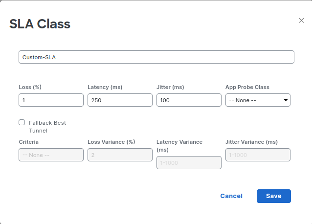
sla-class Custom-SLA
 loss 1
 latency 250
 jitter 100
BFD
Bidirectional Forwarding Detection protocol is used to quickly detect faults between two network devices. In SD-WAN, it is also used to measure loss, latency and jitter. The parameters we use to configure BFD will dictate how fast SD-WAN will detect and react to network problems.
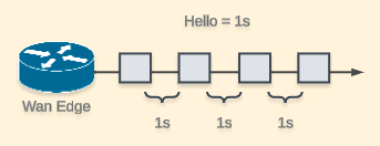
Hello interval
This interval represent how often a BFD echo packet will be sent. It is configured on a per color basis in milliseconds; the default is 1000 ms. This packet will go to the peer wan edge and back, this is how KPIs will be measured for each packet.

sdwan
 interface GigabitEthernetX
   tunnel-interface
   color mpls
   hello-interval 1000 <<<
Each router model has a defined tunnel scale (number of tunnels it can form). Changing the hello interval below 1s lowers the tunnel scale. Keep this in mind to avoid potential problems related to exceeding hardware capacity.
App route poll interval
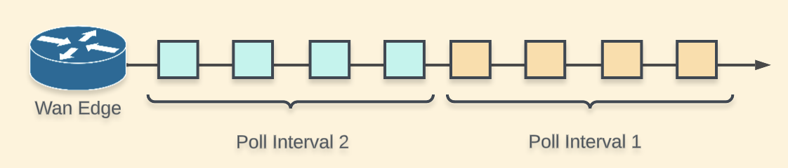
As the wan edge continues to send packets, the poll interval is the timer that will help organize the packets in buckets. These buckets will be used to calculate tunnel statistics. It’s configured on a per box basis (same for all colors).
Let’s say we have a poll interval of 4000 ms. Every 4 seconds a new bucket is built, this bucket will have its own index. Default poll interval is 600,000 ms (10 minutes).
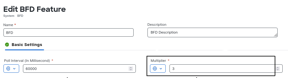
To configure the poll interval
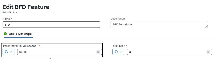
bfd app-route poll-interval 60000
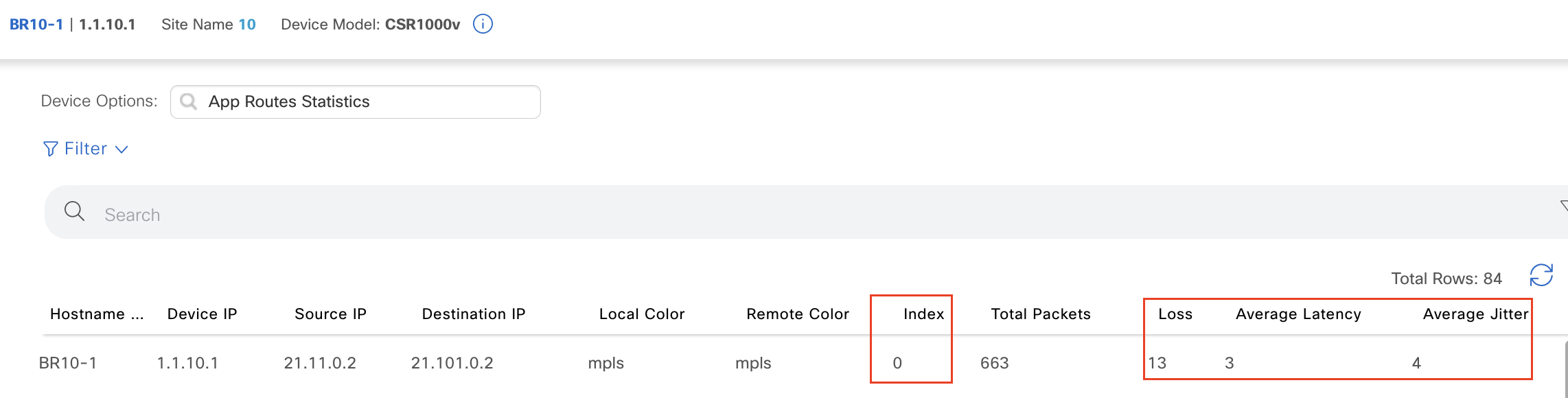
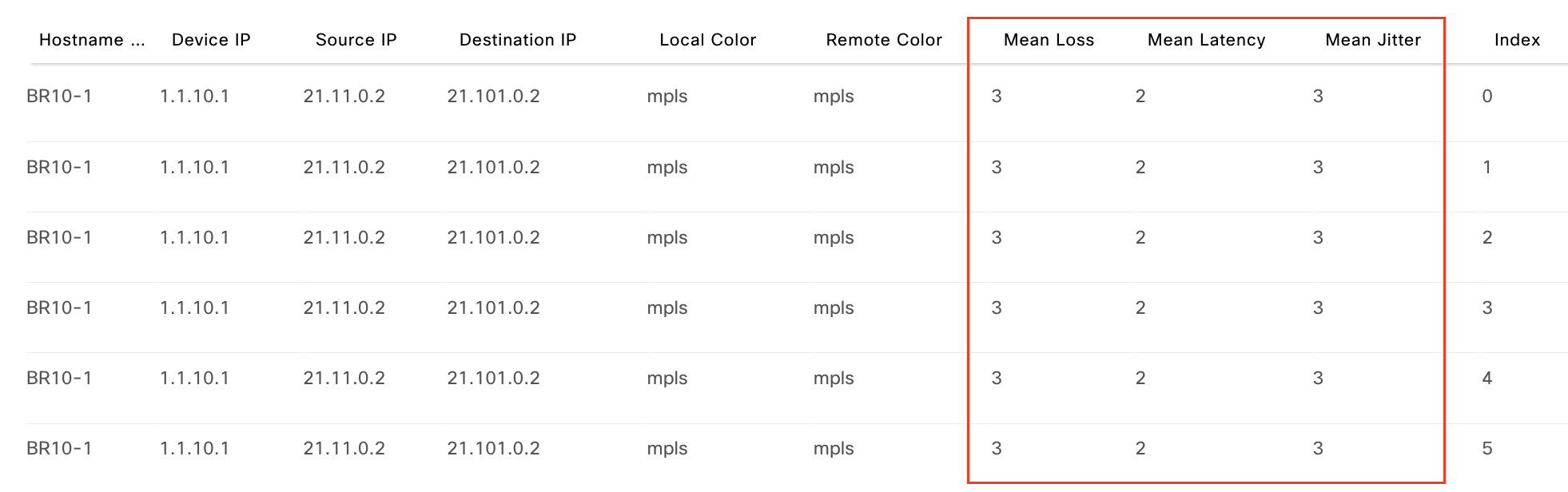
The average loss, latency and jitter will be calculated for each poll interval. We can check this directly on SD-WAN Manager -> Monitor -> Real Time -> App Route Statistics
App route multiplier
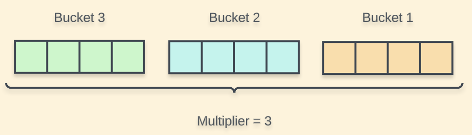
To configure the multiplier
bfd app-route multiplier 3
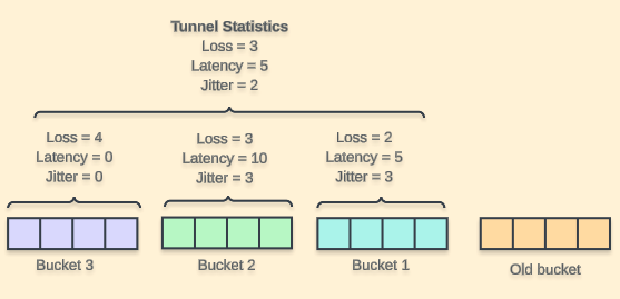
The multiplier will indicate the amount of buckets that will be used to calculate the tunnel statistics that will make the traffic steer when network conditions worsen. For the illustration, a multiplier of 3 is used. By default the multiplier is set to 6.
Notice each bucket contains 4 packets
hello interval (s) x Poll interval (s)
In the real world, 4 packets would be too low. If we take all default values, we would end up with a bucket of 600 packets. Check the AAR Deployment Guide for more details and options.
After filling up all the buckets, tunnel statistics will be calculated.
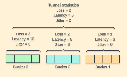
We can visualize the buckets and the mean calculations. Notice the values are the same for all the buckets. Don’t get confused with the avg loss, latency and jitter columns shown before.
This mechanism acts like a sliding window that will discard the oldest bucket to make room for the new one, recalculating tunnel statistics every poll interval.
Configuring AAR policy
Now that we have a better understanding about SLAs and BFD, we can create the rules that will govern the behavior of our AAR policy. This is how it will look on SD-WAN Manager.
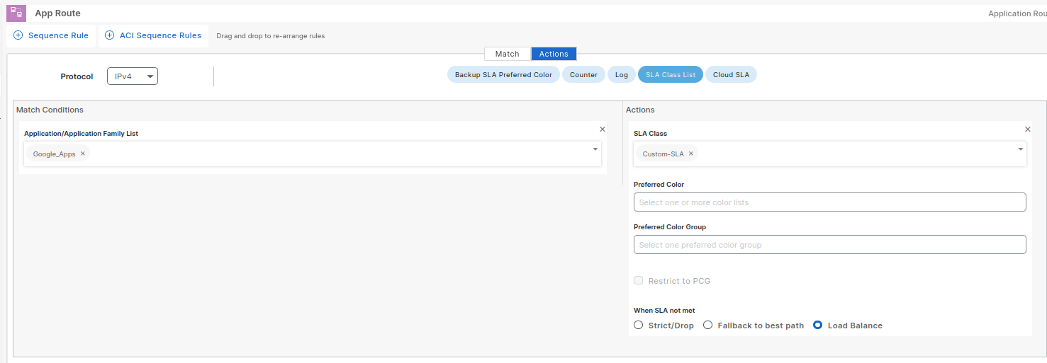
This is probably the simplest form we can configure. Google Apps traffic will be matched and transports matching our Custom-SLA will be used indiscriminately. In other words, if we have 3 different transports and all of them meet the SLA, traffic will be load balanced across them.
What if we want traffic to prefer one of the transports? Well, we can specify a Preferred Color as below:
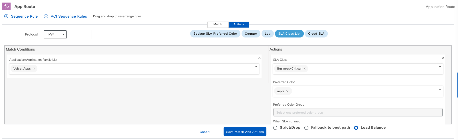
In this sequence, voice apps are matched, and transports’ SLA should match Bussiness-Critical. MPLS will be preferred if it meets the SLA. The action when SLA is not met is set to Load Balance between available colors.
At a first glance, this looks very simple, but there are some details we need to know if we want to fully understand how traffic will behave under different circumstances.
I invite you to read my next post where we will go through some scenarios to get a clear picture. See you there!